Customize Application#
This section provides a detailed walkthrough of building a complete object tracking and smart parking system. It utilizes a combination of technologies designed for ease of use: the Deep Learning Streamer Pipeline Server (DL Streamer Pipeline Server), the visual programming tool Node-RED, and the data visualization platform Grafana. This approach caters to no-code/low-code users, enabling them to create sophisticated analytics solutions with minimal programming.
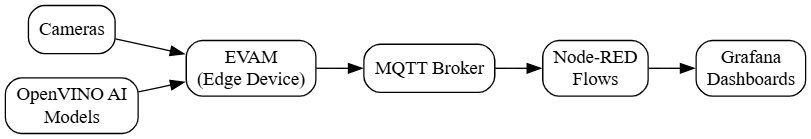
Overall System Architecture#
The system follows a modular architecture:
Video Input: Cameras or video streams provide the raw data.
Deep Learning Streamer Pipeline Server (DL Streamer Pipeline Server): Processes video streams locally using AI models to detect and track objects.
Node-RED: Consumes object tracking data from the DL Streamer Pipeline Server, performs further analysis (like calculating distances), and publishes results.
Grafana: Visualizes the processed data from Node-RED (or a database fed by Node-RED), providing real-time dashboards.
DL Streamer Pipeline Server#
For detailed documentation on DL Streamer Pipeline Server, visit the DL Streamer Pipeline Server Documentation
Overview of DL Streamer Pipeline Server#
The DL Streamer Pipeline Server is a powerful tool designed to process video feeds directly on edge devices. It leverages GStreamer pipelines and OpenVINO-optimized AI models to perform real-time object detection and tracking, minimizing latency and reducing bandwidth consumption.
Key DL Streamer Pipeline Server Components#
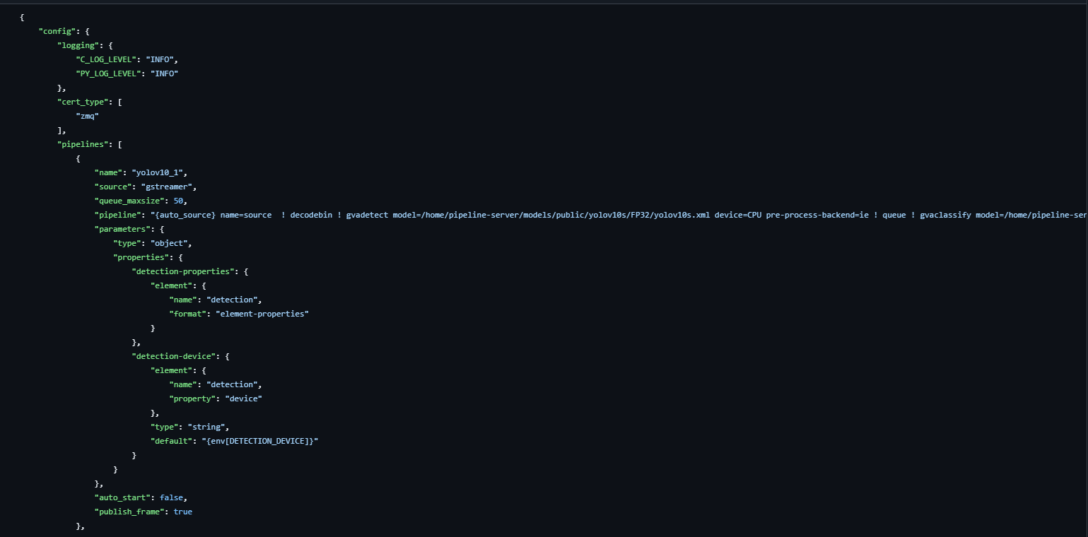
Logging and General Configuration#
C_LOG_LEVEL: INFO- Sets the logging level for C components to “INFO,” which provides useful information about the system’s operations without being overly verbose.PY_LOG_LEVEL: INFO- Similarly, sets the logging level for Python components.
Video Processing Pipelines#
The DL Streamer Pipeline Server utilizes GStreamer pipelines to define the flow of video data through various processing elements.
Object Detection Pipelines (YOLOv10 Series)#
Pipelines like yolov10_1, yolov10_2, etc., are used to identify objects in the video frames.
Pipelines:
yolov10_1,yolov10_2,yolov10_3,yolov10_4How They Work:
Video Source: Uses GStreamer to capture live video.
Decoding & Detection: The pipeline decodes the video stream and uses the
gvadetectelement with a YOLO model (located at/home/pipeline-server/models/public/yolov10s/FP32/yolov10s.xml) to identify objects.Post-Processing:
gvawatermarkadds visual overlays (like bounding boxes) on detected objects.gvametaconvertandgvametapublishprocess and publish the metadata.gvafpscountermonitors the frame rate.
Queue Management: Each pipeline has a queue with a maximum size of 50, ensuring smooth data handling even during high loads.
Control Options:
Auto-Start: Set tofalseso you can start the pipeline manually.Publish Frame: Enabled, allowing the system to output processed video frames for visualization.
Object Tracking Pipelines#
Pipelines like object_tracking_1, object_tracking_2, object_tracking_3, object_tracking_4 are designed to track objects detected by the object detection pipelines.
Pipelines:
object_tracking_1,object_tracking_2,object_tracking_3,object_tracking_4How They Work:
Detection Model: Uses the
pedestrian-and-vehicle-detector-adas-0001model for specialized tracking.Tracking Element: Incorporates
gvatrackwith the settingtracking-type=short-term-imagelessto follow objects over time.Additional Parameters:
Threshold: Set to0.1to balance sensitivity and accuracy.Inference Interval: Controls how often the model analyzes frames.
Benefits: These pipelines help track moving objects (like people or vehicles) across frames, essential for smart parking and other advanced analytics.
Configurable Parameters#
Each pipeline is designed to be user-friendly and customizable:
Detection Properties: Configurable parameters let you adjust the model settings without writing code. Example: The “detection-properties” element defines how the object detection module should behave.
Detection Device: The “detection-device” parameter determines which hardware (e.g., CPU) to use. It uses an environment variable (
{env[DETECTION_DEVICE]}) to make it flexible across different setups.
Messaging Interface (MQTT)#
To share the results of the video analysis with other parts of your system, the DL Streamer Pipeline Server uses a messaging interface based on Message Queuing Telemetry Transport (MQTT):
Publisher Configuration:
Name: defaultType: mqttEndpoint: tcp://0.0.0.0:1883Topics: Messages are published under topics like yolov5 and yolov5_effnet (you can update these as needed).Allowed Clients: All (*), ensuring that any subscribed system can receive the data.
DL Streamer Pipeline Server Workflow#
Capture and Decode: Live video is captured and decoded using GStreamer.
Detection and Tracking: The object detection pipelines analyze each frame to identify objects. The tracking pipelines then follow these objects over time, ensuring that moving objects are continuously monitored.
Data Enrichment and Publishing: Detected objects are enriched with metadata (such as bounding boxes, timestamps, and object types). The processed data is published via MQTT, making it available for dashboards.
Node-RED Flow for Data Processing#
For comprehensive Node-RED documentation, visit the Official Node-RED Documentation
Node-RED is a flow-based programming tool that lets you visually wire together devices, APIs, and online services. This guide demonstrates how Node-RED can be used to process video analytics data from the DL Streamer Pipeline Server for tasks such as object tracking and smart parking. Using a drag-and-drop interface, you can build complex workflows with minimal coding, making it ideal for no-code/low-code environments.
Overview of the Node-RED Flow#
Node-RED is a flow-based programming tool that lets you visually wire together devices, APIs, and online services. This guide demonstrates how Node-RED can be used to process video analytics data from the DL Streamer Pipeline Server for tasks such as object tracking and smart parking. Using a drag-and-drop interface, you can build complex workflows with minimal coding, making it ideal for no-code/low-code environments.
Key Node-RED Components#
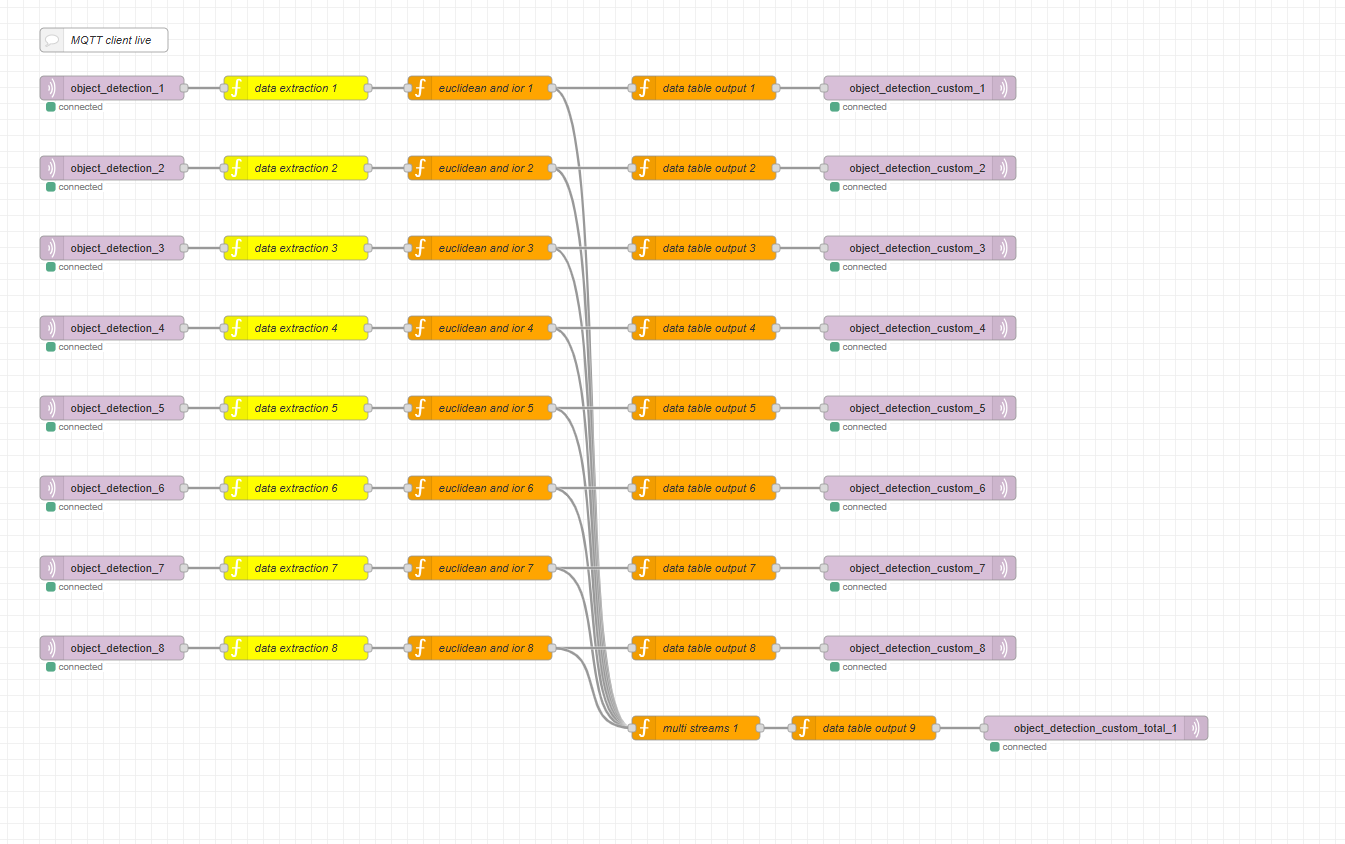
MQTT Input Nodes#
Purpose: To receive real-time object tracking data from DL Streamer Pipeline Server via MQTT. Assume the DL Streamer Pipeline Server is configured to forward its MQTT messages to an MQTT broker.
Configuration Details:
Server Address: 0.0.0.0:1883 (Example - replace with your MQTT broker's address)Topics: For example, object_tracking_1, object_tracking_2, etc.Quality of Service (QoS): 2 (ensuring exactly-once delivery)
Usage: These nodes are the entry points for the data flow. They subscribe to specific MQTT topics, automatically parsing incoming messages for further processing.
Data Extraction Nodes#
Purpose: To extract and filter meaningful information from raw MQTT messages.
Key Tasks:
Parsing the Payload: The node retrieves the list of detected objects.
let payload = msg.payload["objects"];
Fetching Configuration Variables: Retrieve parameters such as object confidence thresholds and target object types from the flow context.
var object_confidence = flow.get("object_confidence");
var target_object = flow.get("target_object");
Filtering and Timestamping: Iterates through the object list, applying filters (e.g., minimum confidence) and appending timestamps.
var date = new Date();
msg.nodered_timestamp = date.toLocaleString();
msg.object_timestamp = date.getTime() / 1000;
Outcome: A structured message containing only the relevant object data, ready for further analysis.
Euclidean and IoR Nodes (Loitering Detection)#
Purpose: To perform advanced spatial analysis, crucial for determining object positions. We’ll focus on a simplified Euclidean distance approach suitable for a low-code environment.
Key Processes:
A. Preprocessing Object Data
Extracting Object Properties: A helper function extracts properties like type, color, ID, and region type from each detected object.
function getObjectData(object_data) {
    let current_object_data = {};
    if (object_data.hasOwnProperty("type")) {
        current_object_data["type"] = object_data["type"];
    }
    // Additional properties like color, license_plate, etc.
    return current_object_data;
}
B. Bounding Box Calculation
Extracting Coordinates: Retrieve bounding box coordinates to understand the object’s location. Assume the bounding box is represented by x1, y1, x2, y2 in the
msg.payload. We’ll use the center point of the bounding box for distance calculations:
let x_center = (msg.payload.x1 + msg.payload.x2) / 2;
let y_center = (msg.payload.y1 + msg.payload.y2) / 2;

msg.object_position = { x: x_center, y: y_center };
Imagine the “smart box” for smart parking again. We said it needs to calculate the distance an object has moved. This is where a little bit of code comes in, but don’t worry, it’s not scary!
Calculating Distance
let distance = Math.sqrt(Math.pow(msg.object_position.x - initialPosition.x, 2) + Math.pow(msg.object_position.y - initialPosition.y, 2));
let distance = ...: This line creates a “variable” calleddistance. A variable is just a named storage location, like labeling a box to put something in. Thedistancevariable will store the calculated distance.msg.object_position.x: Remember,msgis the message containing the object’s information.msg.object_position.xmeans “get the X coordinate from the object’s position information”. Imaginemsg.object_positionbeing like a form, andxbeing one of the fields on that form.initialPosition.x: This is the X coordinate of the object’s starting position, which the smart box remembered earlier.msg.object_position.x - initialPosition.x: This subtracts the starting X coordinate from the current X coordinate. It tells us how far the object has moved horizontally.Math.pow(..., 2): This part squares the result of the subtraction. “Squaring” a number just means multiplying it by itself (e.g., 3 squared is 3 * 3 = 9). We do this to handle positive and negative movements the same way.+: This adds the squared horizontal movement to the squared vertical movement (which is calculated in the same way usingmsg.object_position.y - initialPosition.y).Math.sqrt(...): This is short for “square root”. It “undoes” the squaring we did earlier. The square root of a number is the value that, when multiplied by itself, equals the original number (e.g., the square root of 9 is 3).
Putting it all together: The entire line calculates the straight-line distance between the object’s current position and its starting position. This formula is called the “Euclidean distance,” but you don’t need to remember that! Just think of it as a standard way to calculate distance on a map.
Checking the Time Elapsed
let timeElapsed = msg.object_timestamp - initialTimestamp;
if (timeElapsed >= loiteringThresholdTime) {
    msg.loitering = true; // Object is loitering!
}
let timeElapsed = ...: Creates another variable calledtimeElapsedto store the amount of time that has passed.msg.object_timestamp - initialTimestamp: Subtracts the object’s current timestamp from the timestamp when it started at its initial position. The result is the time elapsed.if (timeElapsed >= loiteringThresholdTime) { ... }: This is a conditional statement. It checks iftimeElapsedis greater than or equal to theloiteringThresholdTimethat we configured.msg.loitering = true;: If the time elapsed is long enough, this line sets theloiteringflag totrue. This tells the rest of the system that the object is loitering!
Outcome: Enhanced object data that includes spatial metrics and a
msg.loiteringflag.
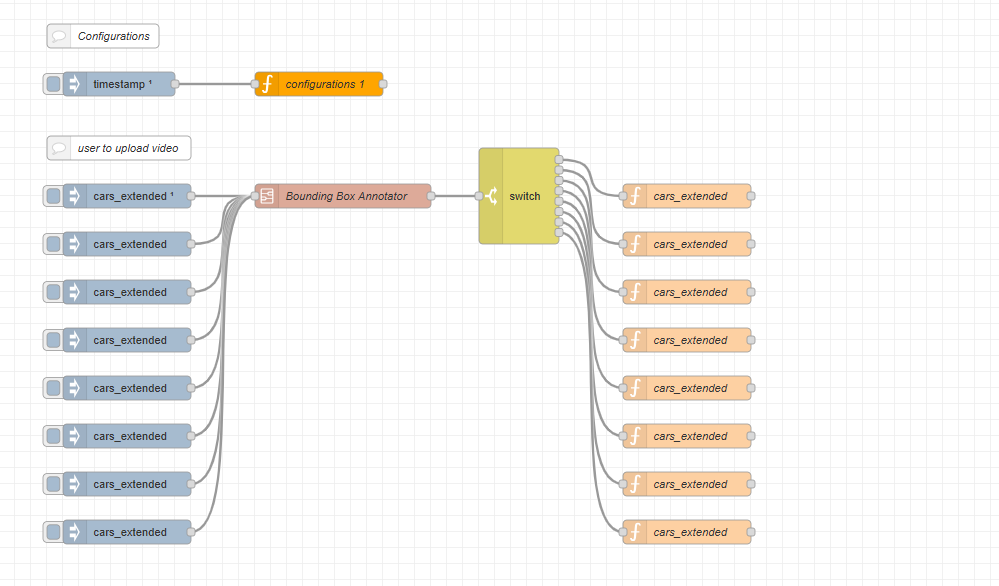
Data Table Output Nodes#
Purpose: To convert processed object data into a structured, tabular format that is easy to read and interpret.
Key Configuration:
Table Headers: Define the columns for output.
var header = ["Zone ID", "Spot ID", "ID", "Status", "Type", "Loitering"];
Data Mapping: Specify which fields from the processed data correspond to each column.
var data = ["video_id", "region_id", "id", "occupied", "roi_type", "loitering"];
Processing Logic:
Iterating Over Objects: The node loops through each detected object, filters out invalid entries, and assigns region names dynamically.
for (let i = 0; i < keys.length; i++) {
    // Determine number of entries, check for valid IDs, etc.
    var region_name = "Region " + payload[keys[i]][data[h]];
    result.payload[region_name] = {};
}
Handling Empty Data: If no objects are detected, the node returns an empty result to prevent errors downstream.
Outcome: A clean, structured JSON object that can be easily consumed by visualization tools or stored in a database.
MQTT Output Nodes#
Purpose: To publish the final processed data, such as loitering status updates, back to an MQTT topic. This allows other systems (like dashboards) to subscribe and react to the data.
Configuration Details:
Server Address: 0.0.0.0:1883Topic: For example, loiter_status_1QoS: 2Retain Flag: Enabled, so that the last message is stored for new subscribers.
Usage: After all processing and formatting are complete, this node publishes the output data, ensuring that downstream services always receive up-to-date information on object status and loitering events.
Node-RED Workflow#
Data Ingestion: MQTT Input Nodes receive live data from the DL Streamer Pipeline Server (relayed via MQTT broker).
Data Processing:
Data Extraction Nodes filter and enrich the data by adding timestamps and applying confidence thresholds.
Euclidean Distance calculation and smart parking.
Data Structuring: Data Table Output Nodes organize the processed data into a clear, tabular format.
Data Publication: MQTT Output Nodes send the final loitering status updates to an MQTT topic, making it accessible to visualization tools (e.g., Grafana).
Grafana Visualization#
For detailed Grafana documentation, visit the Official Grafana Documentation
Overview of Grafana#
Grafana is a powerful, open-source visualization tool that helps you create dynamic dashboards for monitoring real-time data. With Grafana, you can easily visualize the outputs from your the DL Streamer Pipeline Server and Node-RED systems without deep coding skills. Here’s how you can leverage Grafana in your analytics workflow.
Key Grafana Components#
Data Sources#
MQTT Integration: Directly query data from the DL Streamer Pipeline Server or Node-RED endpoints via MQTT datasource.
Dashboards and Panels#
Dashboards: A collection of panels arranged to provide an overview of your system’s performance.
Panels: Individual visualizations (graphs, tables, single-stat panels) that display specific data points.
Setting up Grafana#
Install and Launch Grafana#
Installation: Install Grafana on your local machine or server by following the official Grafana installation guide.
Access: Once installed, access Grafana via your web browser at the designated URL.
Add Your Data Source#
Step-by-Step (Example with MQTT):
Go to
Configuration > Data Sources.Click
Add data sourceand selectMQTT.Enter the connection details (host, port, topic, credentials).
Save and test the connection to ensure it’s working.
Create Your Dashboard#
Dashboard Creation:
Click the
+icon and selectDashboard.Add panels by clicking
Add new panel.Configure each panel with queries to fetch data from your connected MQTT data source.
Use drag-and-drop controls to arrange panels for the best view of your metrics.
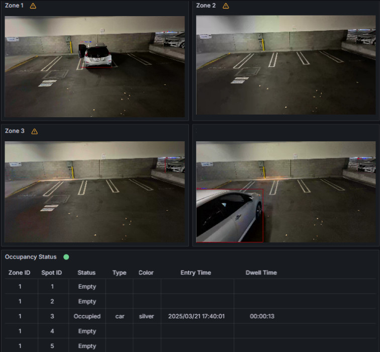
Grafana Use Cases for Object Tracking and Loitering Detection#
Real-Time Object Detection Visualization: Display a graph that shows the number of objects detected per minute to monitor activity levels.
Loitering Event Monitoring: Create a panel that highlights loitering events.
Historical Trend Analysis: Use Grafana’s time-series graphs to analyze trends over days or weeks, helping you identify peak activity times or recurring patterns.
End-to-End Integration#
The system operates as follows:
Video Input: A camera captures video and sends the stream to the DL Streamer Pipeline Server.
DL Streamer Pipeline Server Processing: The DL Streamer Pipeline Server processes the video, detects and tracks objects using its AI models. It publishes metadata about the detected objects (ID, bounding box coordinates, object type, timestamps) to MQTT.
MQTT Bridging (DL Streamer Pipeline Server Configuration): The DL Streamer Pipeline Server is configured to relay the MQTT messages to an MQTT broker. This broker acts as a central hub for the data.
Node-RED Processing: Node-RED subscribes to the relevant MQTT topics. It receives the object metadata, filters the data, calculates the Euclidean distance to determine loitering, and adds the loitering flag to the data.
Grafana Visualization: Grafana directly consumes MQTT topics through its MQTT datasource to create dashboards showing real-time object counts and events.
Data at Each Step:
DL Streamer Pipeline Server Output (MQTT): JSON payload containing an array of detected objects. Each object has properties like
id,type,confidence,x1,y1,x2,y2, andtimestamp.Node-RED Processed Data: JSON payload with the same object properties as above, plus the calculated
object detectionflag and any other derived metrics.
Conclusion#
This guide has demonstrated a complete object tracking and smart parking system using the DL Streamer Pipeline Server, Node-RED, and Grafana. The system provides a balance of edge processing, flexible data manipulation, and powerful visualization. The low-code nature of Node-RED and the user-friendly interface of Grafana make this solution accessible to users without extensive programming knowledge. This allows for quick deployment, easy customization for specific use cases, and scalability to handle multiple cameras and locations.